`WarpKriging`

Description

Create a WarpKriging Object representing a Trend \(+\) GP Model with per-variable input warping. Each input dimension is independently mapped through a learnable transform \(w_j\) before the base kernel is evaluated:

\[ k(\mathbf{x}, \mathbf{x}') \;=\; \sigma^2 \cdot k_{\text{base}}\!\bigl(\Phi(\mathbf{x}), \Phi(\mathbf{x}')\,;\, \theta\bigr), \qquad \Phi(\mathbf{x}) = \bigl[\,w_1(x_1),\, w_2(x_2),\, \dots,\, w_d(x_d)\,\bigr]. \]

All warping parameters are optimised jointly with the GP hyper-parameters \((\sigma^2, \theta, \beta)\) by maximising the marginal log-likelihood.

Usage

Just build the model:

Python

wk = WarpKriging(warping = ["kumaraswamy", "kumaraswamy"], kernel = "matern5_2", noise = None)
# later, call wk.fit(y, X, ..., noise = None)

R

wk <- WarpKriging(warping = c("kumaraswamy", "kumaraswamy"), kernel = "matern5_2", noise = NULL)
# later, call wk$fit(y, X, ..., noise = NULL)

Matlab/Octave

wk = WarpKriging(warping = {"kumaraswamy", "kumaraswamy"}, kernel = "matern5_2", noise = [])
% later, call wk.fit(y, X, ..., noise = [])

or, build and fit at the same time:

Python

wk = WarpKriging(
    y, X,
    warping    = ["kumaraswamy", "kumaraswamy"],
    kernel     = "matern5_2",
    regmodel   = "constant",
    normalize  = False,
    optim      = "BFGS+Adam",
    objective  = "LL",
    parameters = None,
    noise      = None,
)

R

wk <- WarpKriging(
  y, X,
  warping    = c("kumaraswamy", "kumaraswamy"),
  kernel     = "matern5_2",
  regmodel   = "constant",
  normalize  = FALSE,
  optim      = "BFGS+Adam",
  objective  = "LL",
  parameters = NULL,
  noise      = NULL
)

Matlab/Octave

wk = WarpKriging( ...
  y, X, ...
  warping    = {"kumaraswamy", "kumaraswamy"}, ...
  kernel     = "matern5_2", ...
  regmodel   = "constant", ...
  normalize  = false, ...
  optim      = "BFGS+Adam", ...
  objective  = "LL", ...
  parameters = [], ...
  noise      = [] ...
)

Julia

using jlibkriging
# build only
wk = WarpKriging(warping=["kumaraswamy", "kumaraswamy"], kernel="matern5_2", noise=nothing)
# later, call fit(wk, y, X, ..., noise=nothing)

# or build and fit at the same time
wk = WarpKriging(y, X,
                 warping=["kumaraswamy", "kumaraswamy"],
                 kernel="matern5_2",
                 regmodel="constant",
                 normalize=false,
                 optim="BFGS+Adam",
                 objective="LL",
                 parameters=nothing,
                 noise=nothing)

Arguments

Argument	Description
`y`	Numeric vector of response values.
`X`	Numeric matrix of input design.
`warping`	Vector of warping specifications, one per input dimension. See Warping specifications below.
`kernel`	Base covariance model applied in the warped feature space: `"gauss"`, `"exp"`, `"matern3_2"`, `"matern5_2"`.
`regmodel`	Universal Kriging linear trend: `"constant"`, `"linear"`, `"interactive"`, `"quadratic"`.
`normalize`	Logical. If `TRUE` both the input matrix `X` and the response `y` are normalized to take values in the interval \([0, 1]\).
`optim`	Optimisation method used to fit warp and GP hyper-parameters jointly. Possible values are: `"BFGS+Adam"` (bi-level: L-BFGS on \(\log\theta\) inside Adam on the warp parameters — the default), `"BFGS"` (joint L-BFGS-B on all parameters) and `"none"` (keep `parameters` as-is).
`objective`	Character giving the objective function to optimise. Currently `"LL"` (Log-Likelihood).
`parameters`	Initial values and options for the optimiser. Named list / dict with optional entries `"sigma2"`, `"theta"`, `"max_iter_bfgs"`, `"max_iter_adam"`, `"adam_lr"`.
`noise`	Either a numeric vector of per-observation noise variances, `"nugget"` to estimate a homogeneous nugget, or `NULL` (default) for noise-free interpolation.

Warping specifications

Each entry of warping is a string describing the transform for one input variable. Supported forms (see also the Warping Gallery for full examples and plots):

Spec	Description	Params	Details
`"none"`	identity (no warping)	0	→
`"affine"`	\(w(x) = a\,x + b\)	2	→
`"boxcox"`	Box–Cox \(w(x) = (x^\lambda - 1)/\lambda\)	1	→
`"kumaraswamy"`	Kumaraswamy CDF on \([0,1]\): \(w(x) = 1 - (1 - x^a)^b\)	2	→
`"knots(K)"`	piecewise-linear monotone, `K` knots	\(K+1\)	→
`"neural_mono(H)"`	small monotone neural network, `H` hidden units	\(3H+1\)	→
`"mlp(h1:h2,q,act)"`	unconstrained MLP (multi-dim output `q`, activation `act`)	varies	→
`"categorical(L,q)"`	categorical embedding: `L` levels in \(\mathbb{R}^q\)	\(L\cdot q\)	→
`"ordinal(L)"`	ordered positions for `L` discrete levels	\(L-1\)	→
`"mlp_joint(h1:h2,q,act)"`	single MLP taking all inputs jointly	varies	(see `MLPKriging`)

Defaults for omitted sub-arguments: "neural_mono" → "neural_mono(8)", "mlp" → "mlp(16:8,2,selu)", "categorical(5)" → "categorical(5,2)".

Details

The warped representation \(\Phi(\mathbf{x})\) is the concatenation of all per-variable outputs. The GP kernel then operates in this warped space.

The default optimiser is a bi-level strategy: an outer Adam loop updates the warp parameters, while an inner L-BFGS loop optimises \(\log\theta\) with analytical gradients. The variance \(\sigma^2\) and trend coefficients \(\beta\) are concentrated out (computed analytically) at each step.

Reference:

Garrido-Merchán & Hernández-Lobato (2020), Dealing with categorical and integer-valued variables in Bayesian Optimization with GP.
Saves et al. (2023), SMT 2.0: surrogate modelling toolbox with mixed variables support.

Value

An object "WarpKriging". Should be used with its predict, simulate, update methods.

Examples

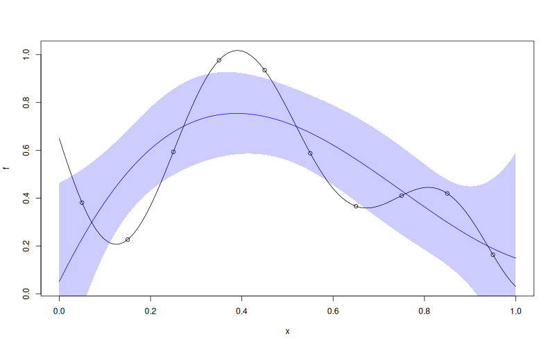
f <- function(x) 1 - 1 / 2 * (sin(12 * x) / (1 + x) + 2 * cos(7 * x) * x^5 + 0.7)
X <- as.matrix(seq(0.05, 0.95, length.out = 10))
y <- f(X)

wk <- WarpKriging(
  y, X,
  warping = "kumaraswamy",
  kernel = "gauss",
  parameters = list(max_iter_adam = "20", max_iter_bfgs = "10")
)
print(wk)

x <- as.matrix(seq(0, 1, length.out = 101))
p <- wk$predict(x, return_stdev = TRUE)
plot(f)
points(X, y)
lines(x, p$mean, col = "blue")
polygon(c(x, rev(x)), c(p$mean - 2 * p$stdev, rev(p$mean + 2 * p$stdev)),
        border = NA, col = rgb(0, 0, 1, 0.2))

Results

* WarpKriging
* data: 10x[0.05,0.95] -> 10x[0.163421,0.976851]
* trend constant (est.): 126.685
* variance (est.): 2.63805e+08
* covariance:
  * kernel: gauss
  * range (est.): 9
  * warpings:
      x0: "kumaraswamy"  →  Kumaraswamy(a=1.01912, b=0.981236)
  * total warp params: 2
  * fit:
    * objective: LL
    * optim: BFGS+Adam

WarpKriging