`MLPKriging`

Description

Create an MLPKriging object for Deep Kernel Learning: a joint multi-layer perceptron (MLP) is applied to all inputs before the GP kernel is evaluated.

\[ k(\mathbf{x}, \mathbf{x}') \;=\; \sigma^2 \cdot k_{\text{base}}\!\bigl(\Phi(\mathbf{x}), \Phi(\mathbf{x}')\,;\, \theta\bigr), \qquad \Phi(\mathbf{x}) = \mathrm{MLP}(\mathbf{x};\, W) \in \mathbb{R}^{d_{\text{out}}}. \]

All MLP weights, GP range parameters, variance and trend coefficients are jointly optimised by maximising the concentrated log-likelihood.

Usage

Just build the model:

Python

mk = MLPKriging(hidden_dims=[32, 16], d_out=2, kernel="gauss")
# later, call mk.fit(y, X, ...)

R

mk <- MLPKriging(hidden_dims = c(32L, 16L), d_out = 2L, kernel = "gauss")
# later, call mk$fit(y, X, ...)

Matlab/Octave

mk = MLPKriging(hidden_dims = [32, 16], d_out = 2, kernel = "gauss");
% later, call mk.fit(y, X, ...)

Julia

mk = MLPKriging(hidden_dims=[32, 16], d_out=2, kernel="gauss")
# later, call fit(mk, y, X, ...)

or build and fit at the same time:

Python

mk = MLPKriging(y, X, hidden_dims=[32, 16], d_out=2, activation="selu",
                kernel="gauss", regmodel="constant", normalize=False,
                optim="BFGS+Adam", objective="LL", parameters=None)

R

mk <- MLPKriging(y, X, hidden_dims = c(32L, 16L), d_out = 2L, activation = "selu",
                 kernel = "gauss", regmodel = "constant", normalize = FALSE,
                 optim = "BFGS+Adam", objective = "LL", parameters = NULL)

Matlab/Octave

mk = MLPKriging(y, X, hidden_dims = [32, 16], d_out = 2, activation = "selu", ...
                kernel = "gauss", regmodel = "constant", normalize = false, ...
                optim = "BFGS+Adam", objective = "LL", parameters = [])

Julia

mk = MLPKriging(y, X, hidden_dims=[32, 16], d_out=2, activation="selu",
                kernel="gauss", regmodel="constant", normalize=false,
                optim="BFGS+Adam", objective="LL", parameters=nothing)

Arguments

Argument	Description
`y`	Numeric vector of response values.
`X`	Numeric matrix of input design.
`hidden_dims`	Integer vector of hidden layer widths, e.g. `c(32L, 16L)`. Defines the MLP architecture.
`d_out`	Output feature dimensionality (dimension of \(\Phi\)). Default `2`.
`activation`	Activation function for hidden layers: `"relu"`, `"selu"`, `"tanh"`, `"sigmoid"`, `"elu"`. Default `"selu"`.
`kernel`	Base covariance kernel in feature space: `"gauss"`, `"exp"`, `"matern3_2"`, `"matern5_2"`. Default `"gauss"`.
`regmodel`	Universal Kriging linear trend in feature space: `"constant"`, `"linear"`, `"quadratic"`. Default `"constant"`.
`normalize`	Logical. If `TRUE` both `X` and `y` are normalised to \([0, 1]\) before fitting. Default `FALSE`.
`optim`	Optimiser. `"BFGS+Adam"` (default) runs a bi-level loop: Adam updates MLP weights while L-BFGS updates \(\log\theta\). `"BFGS"` runs a joint L-BFGS-B. `"none"` keeps `parameters` unchanged.
`objective`	Objective function. Currently `"LL"` (Log-Likelihood).
`parameters`	Optional named list / dict for tuning: `"max_iter_adam"` (default `"300"`), `"adam_lr"` (default `"0.001"`), `"max_iter_bfgs"` (default `"50"`).

Details

The MLP feature extractor \(\Phi : \mathbb{R}^d \to \mathbb{R}^{d_{\text{out}}}\) shares weights across all inputs (cross-variable interactions). This contrasts with WarpKriging, where each input is mapped independently.

The default "BFGS+Adam" optimiser alternates between:

Adam outer loop — updates MLP weights with gradient descent.
L-BFGS-B inner loop — optimises \(\log\theta\) with exact gradients.

\(\hat\sigma^2\) and \(\hat\beta\) are concentrated out analytically at every step.

Value

An object of class "MLPKriging". Use with its predict, simulate, update methods.

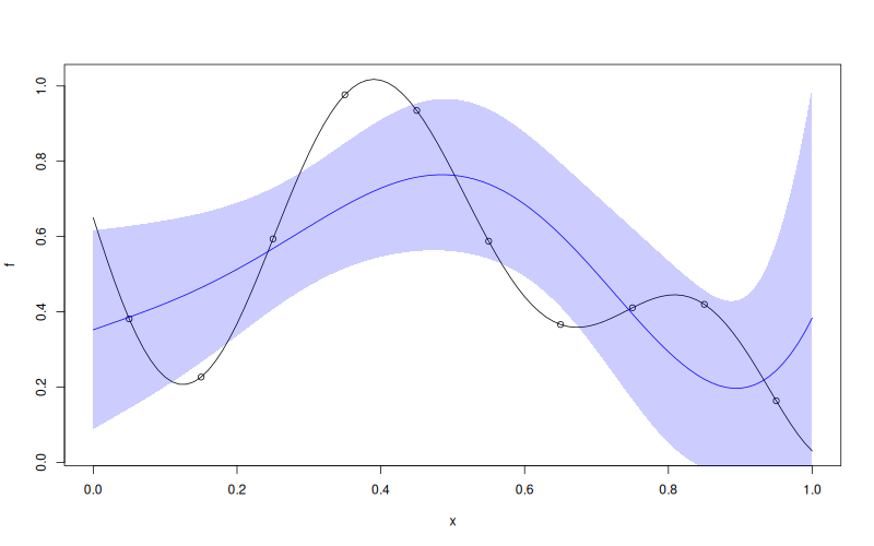
Examples

f <- function(x) 1 - 1 / 2 * (sin(12 * x) / (1 + x) + 2 * cos(7 * x) * x^5 + 0.7)
X <- as.matrix(seq(0.05, 0.95, length.out = 10))
y <- f(X)

mk <- MLPKriging(
  y, X,
  hidden_dims = c(4L),
  d_out = 1L,
  activation = "tanh",
  kernel = "gauss",
  parameters = list(max_iter_adam = "20", max_iter_bfgs = "10")
)
print(mk)

x <- as.matrix(seq(0, 1, length.out = 101))
p <- mk$predict(x, return_stdev = TRUE)
plot(f)
points(X, y)
lines(x, p$mean, col = "blue")
polygon(c(x, rev(x)), c(p$mean - 2 * p$stdev, rev(p$mean + 2 * p$stdev)),
        border = NA, col = rgb(0, 0, 1, 0.2))

Results

* MLPKriging
* data: 10x[0.05,0.95] -> 10x[0.163421,0.976851]
* trend constant (est.): -745.4
* variance (est.): 3.13668e+08
* covariance:
  * kernel: gauss
  * range (est.): 2.88992
  * warpings:
      joint: "mlp_joint(4,1,tanh)"  →  MLPJoint(1 -> 4 -> 1, 13 params)
  * total warp params: 13
  * fit:
    * objective: LL
    * optim: BFGS+Adam

MLPKriging