`WarpKriging::predict`

Description

Predict from a WarpKriging Model Object. The prediction is performed in the warped feature space \(\Phi(\mathbf{x})\).

Usage

Python

# wk = WarpKriging(...)
wk.predict(x, return_stdev = True, return_cov = False, return_deriv = False)

R

# wk <- WarpKriging(...)
wk$predict(x, return_stdev = TRUE, return_cov = FALSE, return_deriv = FALSE)

Matlab/Octave

% wk = WarpKriging(...)
wk.predict(x, return_stdev = true, return_cov = false, return_deriv = false)

Julia

# wk = WarpKriging(...)
p = predict(wk, x, return_stdev=true, return_cov=false, return_deriv=false)
println(p.mean)
println(p.stdev)

Arguments

Argument	Description
`x`	Input points where the prediction must be computed (original input space — warping is applied internally).
`return_stdev`	Logical. If `TRUE` the standard deviation is returned.
`return_cov`	Logical. If `TRUE` the covariance matrix of the predictions is returned.
`return_deriv`	Logical. If `TRUE` the derivatives of the mean and sd with respect to the new input points are returned (computed through the warping via the chain rule).

Details

For new input points \(\mathbf{x}^\star\), the method computes the posterior mean and (optionally) standard deviation / covariance conditionally on the training observations:

\[ \mathbb{E}[y(\mathbf{x}^\star) \,|\, \mathbf{y}] \;=\; \mathbf{f}(\mathbf{x}^\star)^\top \hat\beta \;+\; r(\Phi(\mathbf{x}^\star))^\top R^{-1}(\mathbf{y} - F\hat\beta). \]

The computation uses the warped design \(\Phi(\mathbf{X})\) cached at fit time. Returning derivatives is more expensive than for a plain Kriging model because the chain rule must be propagated through each warp.

Value

A list containing mean and optionally stdev, cov, pred_mean_deriv, pred_stdev_deriv. Note that for a WarpKriging object the prediction is an interpolation at the training points (like Kriging).

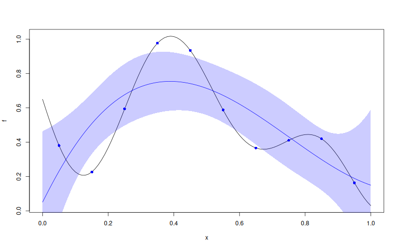
Examples

f <- function(x) 1 - 1 / 2 * (sin(12 * x) / (1 + x) + 2 * cos(7 * x) * x^5 + 0.7)
X <- as.matrix(seq(0.05, 0.95, length.out = 10))
y <- f(X)

wk <- WarpKriging(
  y, X,
  warping = "kumaraswamy",
  kernel = "gauss",
  parameters = list(max_iter_adam = "20", max_iter_bfgs = "10")
)
x <- as.matrix(seq(0, 1, length.out = 101))
p <- wk$predict(x, return_stdev = TRUE)

plot(f)
points(X, y, col = "blue", pch = 16)
lines(x, p$mean, col = "blue")
polygon(c(x, rev(x)), c(p$mean - 2 * p$stdev, rev(p$mean + 2 * p$stdev)),
        border = NA, col = rgb(0, 0, 1, 0.2))

WarpKriging::predict