`WarpKriging::logLikelihoodFun`

Description

Compute the concentrated profile log-likelihood of a WarpKriging model at an arbitrary value of the GP range parameters \(\theta\) (keeping the currently-fitted warp parameters fixed).

Usage

Python

# wk = WarpKriging(...)
wk.logLikelihoodFun(theta, return_grad = True, return_hess = False)

R

# wk <- WarpKriging(...)
wk$logLikelihoodFun(theta, return_grad = TRUE, return_hess = FALSE)

Matlab/Octave

% wk = WarpKriging(...)
wk.logLikelihoodFun(theta, return_grad = true, return_hess = false)

Julia

# wk = WarpKriging(...)
result = logLikelihoodFun(wk, theta, return_grad=false, return_hess=false)

Arguments

Argument	Description
`theta`	Value of the range parameters at which to evaluate the log-likelihood.
`return_grad`	Logical. If `TRUE` the analytical gradient with respect to \(\log\theta\) is returned.
`return_hess`	Logical. If `TRUE` the Hessian is returned.

Details

The warp parameters are held at their currently-stored values. The function evaluates the concentrated profile log-likelihood (with \(\hat\sigma^2\) and \(\hat\beta\) computed analytically) as a function of \(\theta\) alone.

Value

A list with fields logLikelihood, optionally logLikelihoodGrad (vector w.r.t. \(\log\theta\)) and logLikelihoodHess.

Examples

f <- function(x) 1 - 1 / 2 * (sin(12 * x) / (1 + x) + 2 * cos(7 * x) * x^5 + 0.7)
X <- as.matrix(seq(0.05, 0.95, length.out = 10))
y <- f(X)

wk <- WarpKriging(
  y, X,
  warping = "kumaraswamy",
  kernel = "gauss",
  parameters = list(max_iter_adam = "20", max_iter_bfgs = "10")
)
print(wk)
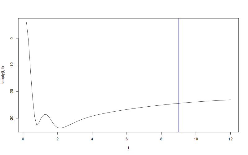
ll <- function(theta) wk$logLikelihoodFun(theta)$logLikelihood

t <- seq(from = 0.2, to = 12, length.out = 101)
plot(t, sapply(t, ll), type = "l")
abline(v = wk$theta(), col = "blue")

Results

* WarpKriging
* data: 10x[0.05,0.95] -> 10x[0.163421,0.976851]
* trend constant (est.): 126.685
* variance (est.): 2.63805e+08
* covariance:
  * kernel: gauss
  * range (est.): 9
  * warpings:
      x0: "kumaraswamy"  →  Kumaraswamy(a=1.01912, b=0.981236)
  * total warp params: 2
  * fit:
    * objective: LL
    * optim: BFGS+Adam

WarpKriging::logLikelihoodFun