Update model objects and simulations
Notations and problems
Throughout this section the following notations will be used for design matrices \(\m{X}\) and vectors of observations \(\m{y}\).
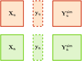
\(\Old{\m{X}}\): contains \(\Old{n}\) observed or “old” design points. The corresponding vector of observations \(\Old{\m{y}}\) is known.
\(\New{\m{X}}\): contains \(\New{n}\) “new” design points at which a prediction or a simulation is made. The corresponding vector of observations \(\New{\m{y}}\) is unknown.
\(\Upd{\m{X}}\): contains \(\Upd{n}\) “update” design points. The corresponding vector of observations \(\Upd{\m{y}}\) is unknown but becomes available at some point where an update step can be performed.
All the design matrices have the same number of columns which is the number of inputs \(d\). The letters \(\told\), \(\tnew\) and \(\tupd\) are not symbols, hence are not italicized.
Note. The notations of this section differ from those of the Predict and simulate section where no “update” design and no “update” observations are used. The correspondence for “old” and “new” objects is \(\Old{\m{X}} \leftrightarrow \m{X}\) and \(\New{\m{X}} \leftrightarrow \m{X}^\star\).
The two following problems are considered here
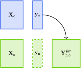
Update a Kriging model object Suppose that a Kriging model has been fitted by using the “old” design \(\Old{\m{X}}\) and the “old” observations \(\Old{\m{y}}\). Later on, the “update” vector of observations \(\Upd{\m{y}}\) corresponding to the “update” design \(\Upd{\m{X}}\) becomes available. We then want to update the fitted Kriging model object. The resulting updated model object should be identical to the model that would be obtained by using the design \(\m{X}_{\told\tupd}\) binding the rows of the two designs \(\Old{\m{X}}\) and \(\Upd{\m{X}}\), along with the vector of observations \(\m{y}_{\told\tupd}\) stacking \(\Old{\m{y}}\) and \(\Upd{\m{y}}\).
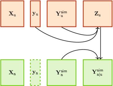
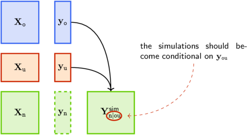
Update conditional simulations Suppose as before that a Kriging model has been fitted by using the “old” design \(\Old{\m{X}}\) and the “old” observations \(\Old{\m{y}}\). Using this model, conditional simulations have been computed for the “new” design points in \(\New{\m{X}}\). This means that \(m\) simulated paths \(\m{y}^{[j]}_{\tnew\vert\told}\) have been computed for \(j=1\), \(\dots\), \(m\), corresponding to the design \(\New{\m{X}}\). Later on, the “update” vector of observations \(\Upd{\m{y}}\) corresponding to the “update” design \(\Upd{\m{X}}\) becomes available. We then want to update the \(m\) simulations so that they become conditional on \(\Old{\m{y}}\) and on \(\Upd{\m{y}}\).
Of course we want each of the two update steps to be faster than the computation “from scratch” of the Kriging model or of the simulations using the observations \(\m{y}_{\told\tupd}\). For the second problem, we rely on the FOXY algorithm of Chevalier et al. [CEG15] allowing the fast update of conditional simulations.
In libKriging the two problems above corresponds to two methods
for the Kriging models classes : update and update_simulate. The
update method updates a Kriging model object. The update_simulate
method can update the conditional simulations that are attached to the
object. These simulations must have previously been attached by using
the simulate method with the corresponding option.
We consider here only non-noisy models for which the notion of path is clear. Hints are given on the noisy case at the very end of this section.
Updating a fitted Kriging model object
Remind that when fitting a Kriging model object with observations \(\Old{\m{y}}\) the costly step is the computation of the Cholesky decomposition of the covariance matrix \(\OldOld{\m{C}} := \m{C}(\Old{\m{X}}, \, \Old{\m{X}})\). This step costs \(O(\Old{n}^3)\) elementary operations.
The Cholesky decomposition can be performed by blocks, see Golub and van Loan [GvL13]. The decomposition of the covariance matrix \(\m{C}(\m{X}_{\told\tupd},\, \m{X}_{\told\tupd})\) takes the form
where the matrices \(\OldOld{\m{L}}\) and \(\UpdUpd{\m{L}}\) are lower triangular with positive diagonal elements. So, \(\OldOld{\m{L}}\) is the Cholesky factor of \(\OldOld{\m{C}}\) hence is available at the update time.
When \(\Upd{n}\) is small relative to \(\Old{n}\), the update is faster than a fit using the observations \(\m{y}_{\told\tupd}\). This is especially true when \(\Upd{n} = O(1)\) while \(\Old{n}\) is large.
Updating simulations
The Kriging weights
An useful tool related to the update of simulations from a Kriging model is the so-called Kriging weights matrix or function.
For a given Kriging model the prediction is linear w.r.t. to the observations and takes the form
where \(\m{W}(\New{\m{X}} \vert \Old{\m{X}})\) is a \(\New{n} \times \Old{n}\) matrix of Kriging Weights. In this notation, the pipe \(\vert\) does not stand as usual for conditioning since \(\Old{\m{X}}\) and \(\New{\m{X}}\) are not random. Yet this recalls that the Kriging Weights depend on the two designs, keeping these in the same order as in our notations for conditioning. Also, it emphasizes the fact that the matrix is a function of the two design matrices and that it does not depend on the GP values.
The matrix of Kriging weights is given by
in the SK case, and by
in the UK case, where \(\widehat{\m{F}}_{\tnew\vert\told}\) is the SK prediction of \(\New{\m{F}}:=\m{f}(\New{\m{X}})\) given the observations \(\Old{\m{F}}\).
Update non-conditional simulations: residual Kriging
Suppose first that we have a Simple Kriging model (with no trend) and that we have performed a non-conditional simulation for a design with two parts \(\Upd{\m{X}}\) and \(\New{\m{X}}\). The \(m\) simulated paths are stored in matrices \(\m{Y}^{\texttt{sim}}_{\tupd}\) and \(\m{Y}^{\texttt{sim}}_{\tnew}\) with dimensions \(\Upd{n} \times m\) and \(\New{n} \times m\).
If at some point the vector \(\Upd{\m{y}}\) of observations becomes available, we can turn the non-conditional simulations in \(\m{Y}^{\texttt{sim}}_{\tnew}\) into conditional ones, say \(\m{Y}^{\texttt{sim}}_{\tnew\vert\tupd}\). In the vocabulary of data assimilation we may say that we are updating the simulations \(\m{Y}^{\texttt{sim}}_{\tnew}\) by assimilating the observations \(\Upd{\m{y}}\).
It is easy to show that the conditional simulations can be obtained by using
The vector \(\Upd{\m{y}} - \m{Y}^{\texttt{sim}}_{\tupd}[\:,\, j]\) may be called a “residual” hence the name of this simulation method. The \(m\) residuals can be stored as the columns of a \(\Upd{n} \times m\) matrix \(\Upd{\m{Z}}\).
This method has been called residual Kriging by Chevalier et al. [CEG15], yet it has been used earlier without this name by Hoffman and Ribak [HR91] and by Durbin and Koopman [DK02].
In the case where an Universal Kriging model is used, one can not obtain non-conditional simulations because the unconditional distribution of \(\m{y}\) is improper. However the residual Kriging method can be used conditionally on the observations \(\Old{\m{y}}\) corresponding to a design \(\Old{\m{X}}\).
Update conditional situations: FOXY
Consider now the case where the simulation is conditional on observations \(\Old{\m{y}}\) corresponding to a design \(\Old{\m{X}}\). We can relax the no-trend assumption of the previous section and simply assume that the distribution of the process conditional on \(\Old{\m{y}}\) is proper i.e., that \(\Old{\m{F}} := \m{F}(\Old{\m{X}})\) has full column rank.
Then the observations \(\Upd{\m{y}}\) at some “update” design points \(\Upd{\m{X}}\) become available, and we want to update the simulations stored in \(\m{Y}^{\texttt{sim}}_{\tnew \vert \told}\)
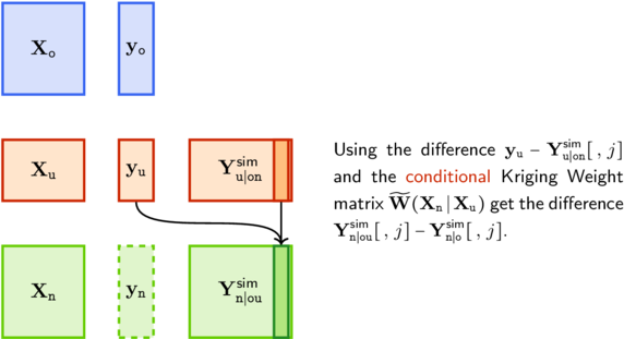
Following Chevalier, Emery, and Ginsbourger we can use the Kriging residual algorithm above but conditionally on \(\Old{\m{y}}\). So we have to consider the conditional covariance Kernel
This kernel expresses as
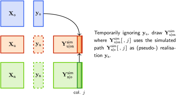
We can then use the residual Kriging algorithm. Yet we do not in general know the value of the simulated paths on the deign points in \(\Upd{\m{X}}\), hence we can not straightforwardly compute the residuals for the design points in \(\Upd{\m{X}}\). So the FOXY algorithm proceeds in two steps
Step 1 Extend the simulated paths to the design points in \(\Upd{\m{X}}\)
Step 2 Use the residual Kriging algorithm with the conditional kernel \(\widetilde{C}(\m{x}, \, \m{x}')\).
Step 1 uses the conditional mean \(\mathbb{E}(\Upd{\m{y}} \vert \m{y}_{\told\tnew})\) and covariance \(\textsf{Cov}(\Upd{\m{y}} \vert \m{y}_{\told\tnew})\), the mean being computed by using the Kriging weights \(\m{W}(\Upd{\m{X}} \vert \m{X}_{\told\tnew})\). In step 2, one uses the Kriging weights \(\widetilde{\m{W}}(\New{\m{X}} \vert \m{X}_{\tupd})\) related to the conditional kernel \(\widetilde{C}(\m{x},\, \m{x}')\). Note that the observations \(\Upd{\m{y}}\) are used only in step 2.
In some case the update design corresponds to a subset of the new design. If so, the step 1 is no longer needed.
Note. Chevalier et al. [CGE14] give update formulas for the Kriging weights.
The noisy case
Recall that simulate for Kriging(noise = <variance vector>) can draw either latent smooth-process paths or noisy observation paths, depending on the selected noise mode. Referring
to the notations used at the end of the Prediction and
simulation section, the simulated non-noisy paths
embed a smooth process part \(\eta(\m{x})\) which is the sum of the
linear trend and the GP components
The simulation essentially generates random draws \(\New{\bs{\eta}}^{[j]}\) for the vector of the \(\New{n}\) values of the smooth process \(\eta(\m{x})\) at the new design points given in \(\New{\m{X}}\).
When the simulate method is used, the random draws are returned as
the columns of a matrix \(\m{Y}_{\tnew \vert \told}^\tsim\). These can
be either: non-noisy, or noisy with the provided noise variance
\(\New{\sigma}^2\). By using the will_update option, the simulations
and the corresponding parameters can be attached to the Kriging model
object. If so, the update_simulate method can be used later. The
“update” observations then provided in \(\m{y}_{\tupd}\) are assumed to
be noisy with a noise \(\sigma_{\tupd}^2\) which can be zero.
Note that when \(\sigma_{\tupd}^2\) is very large, the “update” observations provide only little information about the process part, hence the predictions and simulations from the updated model should be close to those arising from the original model.